


Intro
Key Driver Analysis is a statistical technique that quantifies the importance of a series of predictor variables – known as drivers – in predicting an outcome variable. It is commonly used in the analysis of brand satisfaction and loyalty data, whereupon the predictors are then known as the drivers of satisfaction.
Almost all of the models used in such analysis are correlation or regression-based. So they are prone to suffer from the problem of multicollinearity. This short blog explains what this phenomenon is and how it can affect the results of Key Driver Analysis if “naïve” analysis techniques are used.
Multicollinearity – explained
Multicollinearity refers to a situation in which two or more predictor variables in a linear regression model are highly correlated with each other. When this occurs, it makes it difficult to determine the individual impact of each predictor on the outcomes. This makes it challenging to isolate the impact of each variable and accurately estimate their coefficients. Estimates can change dramatically, depending on which variables have been included.
Multicollinearity is almost always present in customer satisfaction surveys and makes it challenging to build accurate and reliable linear regression models using customer satisfaction data. For, in simple terms, if you are generally happy with one aspect of a brand, say, you are often happy with them all. So, if we derive our importance measure (the regression weights) from linear regression coefficients, then the weights are dependent on which other drivers we include. Worse, you may have drivers appearing to adversely affect the satisfaction levels, when they clearly do not.
Some analysts avoid this problem by using correlation (or squared correlation) between each predictor variable and the outcome variable as the importance weights. Here the problem is that since many factors impact the outcome variable, it is hard to differentiate between them.
Example: Problems with Correlation Analysis
Consider the following dataset with 588 responses to a dentist satisfaction survey. The outcome variable was overall satisfaction, and the scale was 1 being low and 7 being high for this, and each of the 14 drivers.
The base correlations are displayed below with the drivers being ordered from highest to lowest correlation.
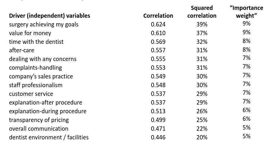
All drivers are highly correlated with overall satisfaction, so it is difficult to tease out which are the most important. Indeed, if we rescale the squared correlations so they sum up to 100% (“Importance weight” column above), there is very little difference between them.
Example: Problems with Linear Regression Analysis
An alternative is to use the coefficients from a linear regression as importance weights. Below is the coefficient from a simple linear regression of overall satisfaction against “overall communication” variable. The regression is significant with an r-squared of 22.2%. (We omit the constant coefficient.)

Now we add the driver complaints-handling into the regression model. The regression is again significant with an increased r-squared of 33.7% but the standardised coefficient for overall communication has decreased by over half.

When adding two more drivers, dealing with concerns and customer service, into the regression model. The regression significance r-squared increases to 38.8% but the coefficient for overall communication has dropped to such a low level that it is insignificant.

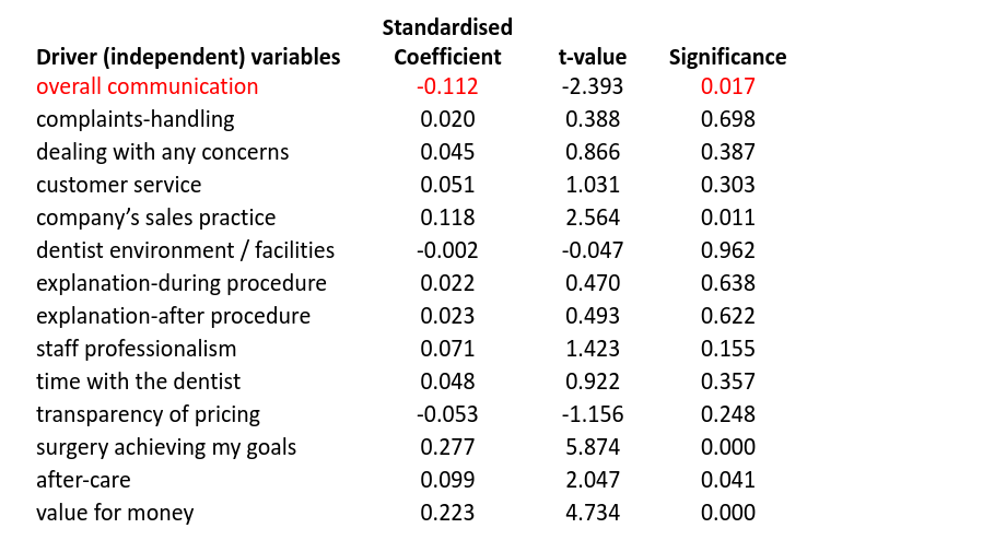
Adding all drivers into the model, we have an r-squared of 50.2% but the coefficient for overall communication is now negative at -0.112, implying that better overall communication leads to lower overall satisfaction. Not only that, it is one of only four significant drivers, so may be reported as important. However, if these results were reported and then acted on, then the dentist could make some very inappropriate decisions.
Conclusion
The above phenomenon is caused by the high degree of multicollinearity in the data. Indeed, no correlation between any pair of drivers is less than 0.500 meaning the drivers are more correlated with themselves than the outcome variable satisfaction.
The regression coefficients are completely misleading when calculated in this way.
This example demonstrates the dangers of using either simple correlations or linear regression as a Key Driver Technique. If you wish to address this problem correctly, we’d recommend using either Kruskal’s Relative Importance Weights (our preference) or Shapley Values.
Importance scores based on these two techniques are produced below. (They have been scaled to sum to 100% in both cases, then sorted).
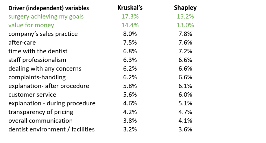
With either case, we have two clear key drivers, easily differentiated from the rest. More importantly, we don’t have overall communication being significant and with a negative sign!