

We needed to estimate the average number of years after purchase various consumer products broke down from a large dataset containing:
- the product type;
- the brand and age of the devices;
- whether or not the devices were still in use;
- if the device was no longer in use, did it breakdown or was it simply replaced.
Such estimates are best provided using survival analysis. We outline below how we applied it in this case, and some of the issues that arose.
Survival analysis
Survival analysis is an area of statistics that studies the (expected) length of time until some particular “event” occurs. This involves estimating the probability distribution of the length of time until the event happens, i.e., constructing a function whereby for each time-period, one can estimate the chances of the event having occurred in the time-period. In our case, the event is the “failure” / “breakdown” of the machine – its (end of) lifetime – whilst time is the age of machine when the particular event happens.
Clearly, we are actually interested in the cumulative probability distribution function, i.e., we wish to know, for any age, the probability that the breakdown has occurred at any point from purchase up to the stated age. For the object of interest is length of time before the event occurs. Indeed, since we are analysing product life-expectancy, it is far more useful to construct what’s known as the survival function S(t); this is the probability of the event not having happened for each age period, i.e., the probability of surviving beyond that age point.
The graph of the survival function is known as the survival curve, and this is what is commonly produced from SPSS, R, or other statistical packages. (The instantaneous probability of breakdown at a time t, given that the machine has survived up to t is called the hazard function, but we won’t focus on that here).
The main technique we used to analyse our data was Kaplan-Meier (KM). This is a well-respected technique that has been used since the 1950s in analysis of clinical survival and product failure rates. It is a non-parametric approach, i.e., it does not yield an age-dependent “formula” to obtain the probability of the event having occurred. However, since most of the data in these sorts of studies is discrete – we have time periods, as opposed to instantaneous moments in time – it is arguably more appropriate. Common parametric distributions include the Exponential and the Weibull, with the latter being the recommended by much of the literature.
As alluded to above, all the survival probabilities we are interested in are conditional probabilities. For, if a product fails during some age-range ‘t’, then it must also have survived through all the previous time periods, i.e.,
P(Breakdown during t) = P(Survive up to t) x P(Fail during t).
Equivalently, we can simply note that the survival function at time ‘t’ is the product of all survival probabilities up to end of age-range ‘t’. This is important since it follows then that we cannot just look at the individual breakdown proportions per time-period to ascertain estimates of life expectancy, irrespective of how precise your estimates of the individual proportions are.
Censoring
The major problem with all survival analysis techniques is the issue of censoring, i.e., cases for which it is not known when the event occurred. In medical studies, this could be because of the end of the study or simply patient drop-out.
In our case, we do not know when a machine breaks down, nor do we know when a machine that was replaced for non-breakdown reasons, when or if it actually breakdowns in the future. Consequentially, our dataset is, in effect, incomplete. If we had the actual ages of breakdown / replacement of every machine, we could easily calculate expected age with confidence intervals. However, we do not. Both the KM non-parametric approach and other survival curve estimations take censoring into account.
In either case, the result of both censoring and the number of products that breakdown / are replaced over time causes the sample size to reduce as time increases. Correspondingly, the standard errors for each survival probability increase as time increases. This makes estimates of survival probabilities past certain time-periods very uncertain.
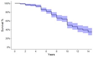
KM survival curve
For any age t, the KM survival point estimate is calculated to be the number of machines that do not breakdown during t divided by the number that were alive at the start of t. Note here that the denominator has removed both the machines that broke down before t and those that have been censored before t (i.e., were replaced for non-faulty reason or were still alive and have age less than t). This is how KM deals with the censoring problem.
The survival function S(t) at time t is then the product of all these point estimates up to time t. Standard errors can be easily calculated from the survival point estimates.
There are two ways of calculating the confidence bounds, either the Greenwood estimates, given by
(S(t) – 1.96*SE, S(t)- 1.96*SE).
or the the log confidence interval, defined to be
(S(t)*exp{- 1.96 * SE / S(t)}, S(t)*exp{+ 1.96 * SE / S(t)}).
We believe the log confidence interval to be more bust, and indeed is the default for the statistical package R uses; SPSS defaults to the Greenwood ones.
Stratification by brand
We needed to produce an overall estimate of expected lifetime for a particular product type. However, it was highly likely that different brands would have expected lifetimes. So, for each product type, we first produced survival curves of the devices grouped by brand, to assess differences.
It was clear by examining the KM survival curves by eye that there were indeed large variations from brand to brand. We therefore needed to consider as many brands as possible separately. However, due to the nature of this type of product data, there were far less older products in the dataset than younger ones. Hence, the confidence bounds around the survival curve became very large as age increased, meaning that we could not be confident that the brands were different over extended time periods. We therefore conducted a set of log-rank tests on the various brand KM survival curves, and considered the devices to be in the “same” brand group unless they differed sufficiently according to the test. We thus produced, for each product type, estimated life expectancies for a small number of brand groups.
Average life expectancy using KM survival analysis
We wished to construct estimates for the average life expectancy of a product, i.e., either the mean or the median length of time before the particular event occurred, plus produce confidence bounds around our estimate.
KM median
The KM median length of time is the age that the probability of survival is less than 50%, and it is generally recommended in the literature to use this measure for the average instead of the mean, if possible. The bounds of the confidence interval of the median is normally defined to be the first time that the lower, respectively, upper, end of any of the confidence intervals for the survival proportions is less than 50%. (The statistical package SPSS uses a different confidence interval for the KM median which we do not believe was appropriate).
However, the problem with using the median was that for some of the product types, this level of breakdown was never reached. So for these products, we had to report the lower bound of the confidence interval of the probability of breakdown at a specified age. In all cases, we reported the (adjusted restricted KM) mean.
KM mean
Irrespective of whether you use a non-parametric or a parametric approach, the mean length of time until the event occurs is equal to the area under the survival curve. However, the standard errors of the mean naturally depend on the approach taken. With KM, they are relatively easily calculated from the survival probabilities; with a parametric curve they are taken from the distribution, assuming the estimates are normal.
Two problems immediately arise when calculating the mean: the maximum expected lifetime is dependent on the age of the oldest product in the survey, and the survival proportion of those who are at this maximum age does not affect the mean. To deal with the first problem, we can produce a series of means called restricted KM survival means. For our final brand estimate, we therefore need to decide which is the most appropriate maximum age to use.
To address the second problem, we used a slight amendment to the KM calculation of the mean: instead of using rectangles to calculate the area, we used trapeziums. This had the advantage of including the last age survival proportion into the calculation and is easy to hand-calculate. We called this the adjusted restricted KM survival mean. Standard errors are not obvious to calculate in this case, but since they are likely to be similar to the original KM estimate, we took an approximate standard error as SE (max age+1).
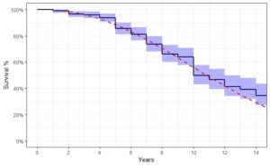
Choosing a maximum age for the adjusted KM mean
Finally, we needed to choose a maximum age for the adjusted restricted KM means.
To guide us in our choice of cap – and to give use some confidence in our KM survival curves – we constructed sets of parametric survival curves on our (merged) brands, using the Weibull distribution. We then plotted both curves on the same graph and visually compared them. Where the curves diverged, i.e., where the Weibull curve lay a long way outside the KM confidence bound, gave us a good guide where to put the maximum age for the adjusted restricted KM mean.