


Standard Excel look-up functions suffer from a problem in that they only match on a single criterion or condition to work, i.e., there is no equivalent to the SQL statement “Where criteria1=A and criteria2=B”.
Have a look at the example below, where you have the Table with the fields: Product, Brand and Sample. There is no direct way using a use a VLOOKUP to get the sample of Product A and Brand 1.
A common way to accomplish this task is to create a new field that is a concatenation of the criteria fields, then use a suitable lookup using this new field as the criterion.
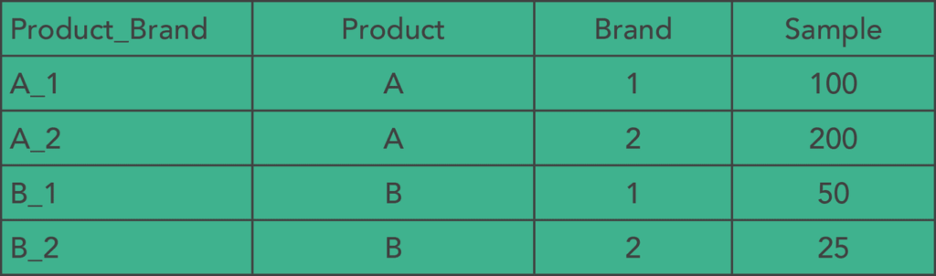
In the example above, we create the field “Product_Brand” and use: =VLOOKUP(“A_1”, Table, 4).
A neater, faster method is to use Excel’s SUMIFS function to look at specific columns where the data that you want lies. In this formula, the Sum column is the column you wish to return the value from, and criteria columns are as required.
In the above example we simply write: =SUMIFS(SampleCol, ProductCol, ’A’, BrandCol, 1) to get the required value.
This approach not only removes the requirement for the new column but is much easier to manage when several criteria are required. Moreover, it will return a zero as opposed to an error when a match is not found.
Note that this approach will only work if you are a returning a single numeric value (i.e., there is only one result for the lookup) – you can’t sum up a text field. Also, be careful to not to use entire columns for the criteria as it can slow up your machine.
Author: Paul Brown, Director